Bayesian Analysis

37.1 Load today’s data
37.2 Background
37.3 Simulation
37.4 Reversing the probability
37.5 Drug testing
37.6 Effect of prior
- 37.6.1 Try it out
37.7 Closing thoughts
- 37.7.1 Limitations
- 37.7.2 Extensions

37.1 Load today’s data

No data to load for today’s tutorial. Instead, we will be using R’s built in randomization functions to generate data as we go.

37.2 Background

Until this point, we have focused on null hypothesis testing. We would set a null, observe some data, determine how likely the data (or more extreme) were, then reject or fail to reject our null. This allowed us to say that something seemed unlikely to be true, but we were never actually able to say how likely it was that the null was true.

We can use a wonderfully ridiculous example to illustrate this:

xkcd xkcd/1132

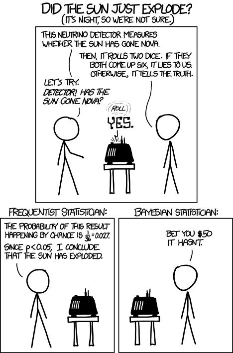
This (admittedly overly simplisic) sort of null hypothesis approach illustrates one of the problems with the approach. Even though it is unlikely to roll two 6’s, it seems even more unlikely that the sun has gone nova. In that case, it seems like we are way more likely to make a type I error (rejecting the null when we shouldn’t) than to make a type II error (failing to reject when we should).

But – how can we address that?

This chapter walks through the very basic levels of an alternative analysis approach that allows us to ask exactly that: Bayesian analysis.

37.3 Simulation

Before we get into the math, let’s start by generating some simulated data. We will use the same game as the last chapter. We will place 15 purple, 20 blue, and 5 orange beads in a (metaphorical) cup. We can save these probabilities in R much like we did in the last chapter:

# Save bead colors
beadColor <- c("purple","blue","orange")

# Save probabilities
prob <- c(15, 20, 5)
prob <- prob / sum(prob)
names(prob) <- beadColor
prob

## purple   blue orange 
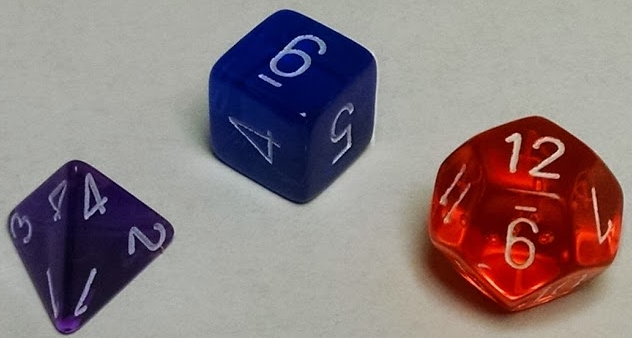
##  0.375  0.500  0.125

Then, we will roll the die of the matching color.

a purple four-sided die if we draw a purple bead
a blue six-sided die if we draw a blue bead, or
an orange twelve-sided die if we draw an orange bead

Dice

So, we need to save the probability of rolling each value from 1 to 12 for each die. To do this, we are going to use a data.frame.

# set probabilities of rolling each value
# note, we need to set from 1 to 12 for each die.
pDie <- data.frame(
  purple = c(rep(1/4 ,  4), rep(0 , 8)) ,
  blue   = c(rep(1/6 ,  6), rep(0 , 6)) ,
  orange = c(rep(1/12, 12), rep(0 , 0))
  )
pDie

	purple	blue	orange
1	0.25	0.1666667	0.0833333
2	0.25	0.1666667	0.0833333
3	0.25	0.1666667	0.0833333
4	0.25	0.1666667	0.0833333
5	0.00	0.1666667	0.0833333
6	0.00	0.1666667	0.0833333
7	0.00	0.0000000	0.0833333
8	0.00	0.0000000	0.0833333
9	0.00	0.0000000	0.0833333
10	0.00	0.0000000	0.0833333
11	0.00	0.0000000	0.0833333
12	0.00	0.0000000	0.0833333

Instead of rolling thousands of dice, we will let R do it for us. For this, we will develop a loop. Each time through, we will draw (sample) a bead then roll the appropriate die. Note that we are using the color of the bead to select a column from pDie in each roll.

# Initialize variables
bead <- character()
die  <- numeric()

for(i in 1:13567){
  # Draw a bead
  bead[i] <- sample(beadColor,
                    size = 1,
                    prob = prob)
  
  # Roll that color die
  die[i]  <- sample(1:12,
                    size = 1,
                    prob = pDie[, bead[i] ])
}

Then we can look at outcomes. Because I like keeping things in order, I am going to make bead into a factor and set the label order to match the colors we set above. This step is not necessary, but can be helpful.

# Make bead a factor for nicer printing
bead <- factor(bead, levels = beadColor)

Then, we can save the outcomes as a table:

# Save the outcomes for easy checking
outcomes <- table(die,bead)

	purple	blue	orange
1	1262	1168	148
2	1295	1156	125
3	1245	1139	156
4	1227	1123	133
5	0	1134	134
6	0	1132	141
7	0	0	129
8	0	0	133
9	0	0	146
10	0	0	148
11	0	0	147
12	0	0	146

Now we have some data to refer back to to check our calculations.

37.4 Reversing the probability

In the last chapter we used the conditional probabilities of rolling a number given that we knew what color the die we rolled was. But now, we want to ask a slightly different question. We want to know the probability that we have certain color die given that we know we rolled a particular value. To make a concrete example:

What is the probability that the die we rolled is purple (four sided), given that we rolled a 1?

We know that our probabilty of rolling a 1 given that we have a purple die is ¹/₄, and we can write that as p(1|purple) = ¹/₄. But, now we want to know the p(purple|1). How can we get there?

37.4.1 Try a null hypothesis

If we were to use null hypothesis testing, we would set a null hypothesis and see if we can reject it. If we are testing dice, we would likely set a 6-sided die (like our blue die) as the null. We would also likely do this as it is the most common bead color in the cup. So, let’s set that up:

H₀: The die is a fair 6-sided die

H_a: The die is not a fair 6-sided die

Right away, you may notice a problem: neither of these tells us anything about the die being purple. But, let’s try this anyway. What is the probability of rolling a one given that we are rolling the blue die (our H₀)?

It is ¹/₆ or 0.1667, and because a 1 is the furthest you can get (in one direction) from the expected mean, this is our one-tailed p-value. This is larger than 0.05, our normal α threshold, so we fail to reject the null hypothesis. But … does that mean the die is definitely fair?

Hopefully by this point, you know that the answer is NO! All we know is that we can’t say that the die is unlikely to be fair. However, that isn’t really what we were asking.

If we simply relied on the null hypothesis test we might be forced to conclude that we can’t tell if the die is fair or not. We can do better.

37.4.2 Look at the simulation

Let’s look again at our outcomes. Here, I am just going to focus on the first row, as that is the only part we are interested in: it has all the ways that we generated our observed values.

outcomes[1, ]

	purple	blue	orange
1	1262	1168	148

From this, what can we see? The purple die is, by a small margin, the most common die rolled when we got a 1.

In fact, we can calculate exactly how often we rolled a purple die given that we got a 1 – which is exactly what we were interested in to start. All we need to do is take the number of purple 1’s we rolled, divided by all of the ones we rolled.

outcomes[1, "purple" ] / sum(outcomes[1,])

## [1] 0.4895268

This shows that about half of the time that we rolled a 1, we had rolled a purple die. That is a lot different than what the null hypothesis test let us say.

Surely, there is a way that we can calculate that without having to run the full simulation.

37.4.3 Applying probabilities

Of course there is. We can use the same approaches that we have learned all along for dealing with probability. Specifically, think carefully about what we (intuitively) did when dealing with numbers, and apply the probabilities to get there.

Perhaps the simplest place to start is to ask the probability of drawing a purple and rolling a one. For this, we turn to our general multiplaction rule, and use the conditional probability:

p(purple & 1) = p(purple) * p(1 | purple)

p(purple & 1) = 0.375 * ¹/₄

And, if we plug this into R:

pPurpleOne <- prob["purple"] * 1/4
pPurpleOne

##  purple 
## 0.09375

So, this gives us something like the top of the equation that we had before. However, we also want to know the probability of getting a 1 in any fashion. This is the same thing as adding up all of the ones from the simulation. For that, we just need to take the sum of the probability of rolling a one and each color.

p(1) = p(purple) * p(1|purple) + p(blue) * p(1|blue) + p(orange) * p(1|orange)

In R, we can type this all out (similar to what we did with conditional probability).

pOne <- prob["purple"] * 1/4 +
        prob["blue"]   * 1/6 +
        prob["orange"] * 1/12
pOne

## purple 
## 0.1875

Now, we can combine those together:

pPurpleOne / pOne

## purple 
##    0.5

This is saying that the probability that we have a purple die given that we know we rolled a 1 is 0.5. Which very closely matches the observed proportion of 0.49.

37.4.4 Bayes Theorem - the math

All we did above was apply what we observed to the probabilities and ask: what is the probability of drawing a purple and rolling a one divided by the probability of rolling any 1. In mathematical notation, that looks like:

\[ \text{p(purple | 1)}= \frac{\text{p(purple & 1)}}{\text{p(1)}} \]

We further know that we can calculate the probability of a purple and a one using conditional probability:

\[ \text{p(purple | 1)}= \frac{\text{p(purple)} \times \text{p(1 | purple)}}{\text{p(1)}} \]

This may seem like a trivial example, but it is actually incredibly illustrative of the general concept. First, it illustrates the (rather severe) limitations of null hypothesis testing. Our large p-value in the above section didn’t help us at all (we will see in a moment that often a small value may not help either). Second, the formula we developed above is entirely generalizable. For any two events, A and B, we can re-write the formula as:

\[ \text{p(A | B)}= \frac{\text{p(A)} \times \text{p(B | A)}}{\text{p(B)}} \]

This formula now applies to any two events we can imagine. For most of our purposes, we will treat our hypothesis as event “A” and the observed data as event “B”. That means that the formula further becomes:

\[ \text{p(H}_i \text{ | data)}= \frac{\text{p(H}_i \text{)} \times \text{p(data | H}_i \text{)}}{\text{p(data)}} \]

So, for any hypothesis (H_i above), we can calculate how likely it is to be true given that any observed data occured, as long as we know:

An initial probability of H_i before observing the data, which is generally called the prior probability
The probability of generating the data given that H~i is true, which may be any probability function, and
The probability that the data would have occurred under any of the hypotheses being investigated, which requires that we have a prior and a conditional probability of generating the data for each of our hypotheses as well.

The result (p(H_i|data) ) is generally called the posterior probability, as it is the probability of that H_i is true given that the data occurred. This is a much more powerful statement than the ability (or failure) to reject some null hypothesis. There are (of course) limiations, and those are discussed at the end of this chapter.

37.4.5 Try it out

What is the probability that you rolled an orange die given that you rolled a 6?

Check your answer to make sure that it is similar to the outcomes of your simulation. My simulation yielded: 0.111

37.5 Drug testing

Imagine that 1% of the audience for this tutorial are drug users, and that we randomly sample some of them to be screened for the drug. For this scenario, let’s imagine that the testing is 99% accurate. Drug testing, just like medical testing or null hypothesis testing, has two ways of being accurate. For drug and medical testing (e.g., testing to see if a patient has a disease) we generally refer to these as:

Sensitivity, the probability of correctly identifying a positive, and
Specificity, the probability of correctly identifying a negative

For the drug test, let’s say that it has a sensitivity of 99% (meaning it will call a false negative in 1% of actual users) and specificity of 98% (meaning it will call a false positive in 2% of non-users).

The question then is: what is the probability that someone with a postive test is actually a drug user?

Think for a moment about this.

What do you think the probability is?

Most people will, before encountering Bayesian methods, say something like 99% because that is the listed accuracy of the test.

If we were to apply a null hypothesis approach, we would say that there is only a 2% chance that a non-user would test positive, making our p-value 0.02. Therefore, we would reject the null-hypothesis that the person is a non-user and conclude that they are likely a user.

Worse yet, we may say that there is only a 2% chance of generating the data given that the null of a non-user is true, so we are 98% confident that the person is a drug user. Hopefully we know that this is not what a p-value means, but that was one of the misconceptions that many students (and faculty, and others) bring to p-values.

37.5.1 What does probability mean here

We are asking about the probability that a given person that tested positive is a drug user. However: does that even make sense? The person either is or is not a drug user. So, in what sense can we talk about a probability.

One way to think about probability in these cases is to imagine many, many trials. Then, instead of asking “what is the probability that this person is a drug user?”, we can ask, “what proportion of positive tests are drug users?”

Not only can this help to re-frame the question, but now we can calculate a simple “simulation” using the given values. For this, you can use any numbers, but it tends to make the arithmetic easier to pick round numbers. Let’s imagine that we test 10,000 individals. First, how many of them are acutally drug users?

Well, 1% of 10,000 is 100. So, 100 people are actually drug users. Of these, how many will test positive?

Our test has a 99% sensitivity, so 99 of the 100 will test positive.

Next, of the 9,900 non-users (10,000 minus our 100 users), how many of them will test positive?

With 98% specificity, 2% of non-users will test positive. This means that 198 (0.02 * 9,900) non-users will test positive.

Putting that all together, 99 drug users will test positive and a total of 297 people will test positive. That means that only one-third of all positive tests are from drug users. A far cry from the 90-some percent that many of you likely initially thought.

37.5.2 Apply Bayes

You may have noticed that what we just did sounds a lot like the Bayes’ Theorem from above:

\[ \text{p(A | B)}= \frac{\text{p(A)} \times \text{p(B | A)}}{\text{p(B)}} \]

We can plug in our probabilities to the equation to apply it to this example:

\[ \text{p(user | positive)} = \frac{\text{p(user)} \times \text{p(positive | user)}}{\text{p(positive)}} \]

This says that our posterior probability of being a user given that the person had a positive test is: the probability of getting a positive test and being a user (our prior times the conditional probability of getting a positive test if the person is a user) divided by the probability of getting a positive test (regardless of use status). We can plug this in to R as:

# Calculate posterior
0.01 * 0.99 / sum(0.01 * 0.99,
                  0.99 * 0.02)

## [1] 0.3333333

Which gives us the same result as our imagined simulation above.

37.5.3 Try it out

Meningitis is a deadly disease that can stike quickly. It is especially prevalent in places where lots of people live in close proximity, and major outbreaks have happened on college campuses in the past.

In one attempt to address this, many colleges mandated that all students get tested for meningitis annually. We know the following things about meningitis:

The rate of occurence is approximately 10 in 100,000 (0.0001) among college students in general
The test is 99.9% sensitive (99.9% of people with meningitis test positive)
The test is 99% specific (99% of people without meningitis test negative)

Given that a random student tested positive, what is the probability that ze actually has meningitis?

You should get an answer of a little less than 1%.

37.5.4 Why this matters

This may seem like an odd thing to be thinking about, but it is actually quite important. Meningitis kills hundreds of thousands of people per year. So, a positive test is likely to send the individual, and their campus community, into a bit of a panic. If less than 1% of them actually have the disease – that panic is probably misplaced (and should be avoided).

The same is true for all tests like this. Cancer tests have similar rates, and it is important that patients (and their doctors) understand that a positive test may not that they have cancer. It may not even mean that they are more likely to have cancer than not. Medical decisions depend on understanding this.

Similarly, routine drug tests have been proposed for everything from employment to government assistance. It is important to understand the rates, and what they mean, before beginning this testing. In our drug testing example, two-thirds of positive tests were for people that we not actually users. Policy decisions must take this into account when deciding how to handle positive results.

37.6 Effect of prior

As you have likely noticed, the effect of the prior ( p(A) ) can be rather substantial. Changing it can (and should) change our posterior ( p(A|B) ).

\[ \text{p(A | B)}= \frac{\text{p(A)} \times \text{p(B | A)}}{\text{p(B)}} \]

Let’s return to our drug testing scenario. This time though, let’s set the population rate of drug users at 10% instead of 1%. The 99% sensitivity and 98% specificity can stay the same. Now, given a positive test, what is the probability that the person is drug user?

We can copy our code for Bayes’ Theorem from above, changing our prior from 0.01 to 0.1:

# Calculate posterior
0.1 * 0.99 / sum(0.1 * 0.99,
                 0.9 * 0.02)

## [1] 0.8461538

Now, given a change in the population rate (our prior) we find that 84.6% of positive tests are from actual drug users. Nothing about the test changed – only our prior did, but it more than doubled the posterior probability that a person is a drug user given that they tested positive.

Some critics argue that this is a draw back of Bayesian analysis (for an example, see this blog post but note the rebuttals in the comments). However, proponents (myself included) argue that this is a benefit of Bayesian approaches (for an example, see this long rebuttal to the above blog post). By being explicit about priors, we are prevented from arbitrarily assigning them.

In our drug testing example, we could use real world rates of drug use as our priors (the rates used are close to the true rates for cocaine and marijuana respectively). More importantly, if we didn’t know the population rate, we could be explicit about that and test the effects of different priors. All statistics rely on assumptions, but for null hypothesis testing, those assumptions are often hidden. Bayesian priors need to be justified to be valid, and they can be explictly tested to see their impact.

37.6.1 Try it out

Return to the meningitis example. Imagine that, after deciding not to test everyone on campus based on the analyis above, a college campus has a confirmed case of meningitis. Given that meningitis exists on campus, the population rate of potentially ill students increases dramatically. For the sake of simple arthimetic, let’s say that, given that meningitis is confirmed on campus, 1 in 1000 (0.1%) other students will get meningitis.

Keeping the testing information the same, what is the posterior probability that a student has meningitis given that they tested positive on a campus that has a confirmed case of meningitis?

You should get an answer a little under 10%.

Now, might testing be more appropriate?

37.7 Closing thoughts

Bayesian analysis is an incredibly broad field and can not be thoroughly covered in a single chapter. In this section, I will jot down a few thoughts and teasers about what else is possible. Hopefully it encourages you to consider these methods as you move on. It may be that they are great methods for research you do, or that this encourages you to seek out an advanced course that covers these things more explicitly.

37.7.1 Limitations

Bayesian analysis has a number of limiting factors, though (as a Bayesian) I’d argue that these are becoming less limiting as more people adopt the methods and the tools and technology advance. Having to identify priors, establish probability distributions, and actually crunch the numbers all limit the entry into Bayesian statistics.

Perhaps the strongest limitation is specifying good priors. While the above priors seemed relatively straight forward to assign, those are exceedingly simple examples. Often, instead of just asking “which of these dice am I rolling?” we may instead be asking “what is the probability that the die I rolled comes up 1 is?” These are related questions, but the later requires that we specify a prior that could land anywhere between 0 and 1, rather than just at a handful of previously identified points.

This is only complicated when models grow more complex, such as when estimating the mean of a distribution or handling multiple variables (such as multiple linear regression). Distributions that work well for this are being further developed, but it can still be especially challenging for someone new to the field.

Even after the priors are set, it is still necessary to calculate the probability of the data given each of the possible priors. For some methods, this seems easy enough. For example, if we were asking about our dice example, it would be easy to use what we know about binomial probability to calculate the probability of rolling any series of values. However, this is complicated as more distinct priors are addded or as the model grows more complex. Like specifying priors, this is overcomable, but it is still a challenging task for novices to the methods.

Finally, Bayesian methods require a lot of compuational resources. While the examples that we had in this chapter used straghtforward arithemetic, many Bayesian analyses require massive sampling loops and extensive calculations. 20 years ago, this made all but the simplest calculations impossible. Now, however, the computer (or even phone) you are viewing this tutorial on is far more powerful than anything in use 20 years ago. This does not make the task easy, but it does make it approachable.

37.7.2 Extensions

As mentioned above, Bayesian methods can be applied any where that we can specify a prior and a conditional probability of the data given each considered hypothesis. This means that any traditional statistical analysis can be replaced by a thorough Bayesian approach.

While the methods for Bayesian analysis have generally focused on complicated situations such as reconstructing massive phylogenies from sparse data, they can also be applied to things as simple as a t-test. For a great example of that, take a look at the website of John Kruschke. It includes a link to a paper entilted: “Bayesian estimation supersedes the t test,” which walks through several common scenarios where a Bayesian method dramatically outperforms the traditional t-test, including the ability to accept the null – something that we can never do with traditional null hypothesis testing.

Several tools are also being developed to make Bayesian methods more accessible to entry-level users. This includes a large number of R packages for Bayesian methods. I have also started developing a small R package to implement the introductory level methods from the fantastic Bayesian text book: Doing Bayesian Data Analysis by John Kruschke.

These methods are emerging, and are likely to continue expanding in the coming years. As greater understanding of the methods is developed, more and more data analysis will involve Bayesian approaches. The basic underlying thinking of Bayesian analysis is already necessary in every aspect of bioinformatics, and it seems likely that (especially as data expands) the methods will become common in other field as well.

An introduction to statistics in R

A series of tutorials by Mark Peterson for working in R

Chapter Navigation

Search these chapters

Bayesian Analysis

37.1 Load today’s data

37.2 Background

37.3 Simulation

37.4 Reversing the probability

37.4.1 Try a null hypothesis

37.4.2 Look at the simulation

37.4.3 Applying probabilities

37.4.4 Bayes Theorem - the math

37.4.5 Try it out

37.5 Drug testing

37.5.1 What does probability mean here

37.5.2 Apply Bayes

37.5.3 Try it out

37.5.4 Why this matters

37.6 Effect of prior

37.6.1 Try it out

37.7 Closing thoughts

37.7.1 Limitations

37.7.2 Extensions